“The eye is not a camera. It is a brain peripheral.”
Before we can talk about ACES, LUTs, or grading, we have to talk about the hardware we were born with. We tend to trust our eyes implicitly. If we see a color, we assume it is “real.” But as a biologist, I have to tell you: your eyes are terrible scientific instruments. They are inconsistent, they auto-balance without asking, and they are easily tricked by simple changes in lighting.
Yet, they are the only reference we have. To master digital color, we first need to understand the signal chain of biological color.
1.1 The Source: Physics of Photons
Visible light is just a narrow slice of the electromagnetic spectrum, roughly 380nm to 780nm. It behaves as both a wave and a particle, defined by the relationship between its wavelength ($\lambda$) and frequency ($\nu$):
\[c = \lambda \nu\]Where $c$ is the speed of light (~299,792,458 m/s).
When we talk about a light source on set, we usually describe it with a single number: Correlated Color Temperature (CCT), like “3200K”. This is a dangerous oversimplification. CCT only tells you the color of the light, not the quality of the spectrum. To see the quality, we need the Spectral Power Distribution (SPD).
The LED Problem: Continuous vs. Discontinuous
Tungsten (Blackbody): A smooth, continuous curve. It rises gently from blue to red. It contains information at every single wavelength.
LED (Discontinuous): A sharp blue spike (the pump) and a broad yellow/green hump (the phosphor).
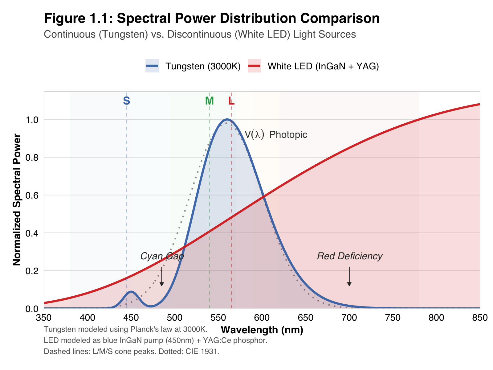
Notice the “valley” in the cyan range and the drop-off in deep reds? That is missing data. If a specific skin tone relies on reflecting 660nm red light, and your LED source isn’t emitting 660nm light, that color simply does not exist in your scene.
Metamerism Failure & The CRI Trap
This leads to the DIT’s nightmare: Metamerism Failure. Two colors might match under Tungsten but look completely different under LED.
Interactive figure in development. It will be published only when it has a cited source or an original, documented demonstration.
We often rely on CRI (Color Rendering Index) to check this, but CRI is flawed. It only samples 8 pastel colors (R1-R8).
The Trap: An LED can have a CRI of 95+ and still make skin look dead because it fails at R9 (Saturated Red).
The Solution: For cinematography, always verify R9, R13 (Skin Tone), and R15 (Asian Skin Tone).
1.2 The Lens & Retina: Variable Resolution
Before light hits the sensor, it passes through the lens, which acts as a UV filter (protecting the retina). The signal then hits the “sensor plane”—the retina. Unlike a camera sensor with uniform resolution, the eye relies on Variable Resolution.
The Fovea vs. The Periphery
The Fovea: A tiny central pit (~2° field of view) densely packed with cones (~200,000 cones/mm²). This is the only place you see high-resolution color.
The Periphery: The rest of the retina. Low resolution, rod-dominant, colorblind, but highly sensitive to motion.
Interactive figure in development. It will be published only when it has a cited source or an original, documented demonstration.
Filmmaking Application: We scan scenes rather than capturing them whole. When composing a shot, you are essentially guiding the viewer’s fovea. If visual info exists in the corner without a leading line, the viewer biologically cannot see it in detail.
1.3 The Photoreceptors: Rods & Cones
Our “sensor” has two distinct modes of operation.
The Cones (Photopic Vision)
We are trichromats with three cone types, defined by peak sensitivity:
- L (Long): ~565nm (Red-Yellow)
- M (Medium): ~540nm (Green)
- S (Short): ~445nm (Blue-Violet)
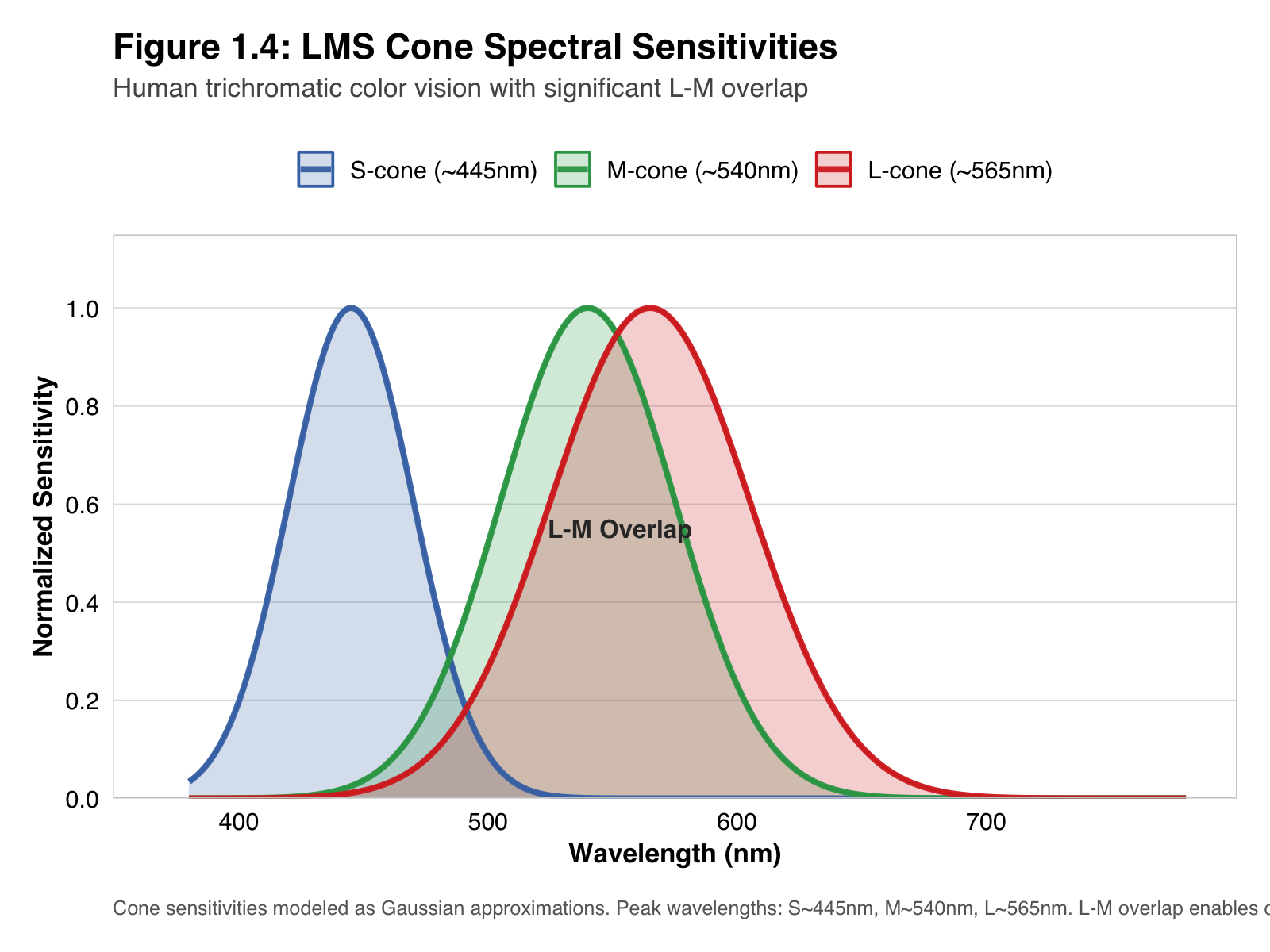
Crucial Insight: The L and M curves overlap significantly. This “Opponent Process” design means the brain must calculate difference signals ($L-M$) to distinguish red from green. This is biologically expensive and explains why we are so sensitive to skin tone shifts.
The Rods (Scotopic Vision) & The Purkinje Effect
In low light, cones shut down. Rods take over, peaking at ~505nm (Blue-Green) and becoming blind to red.
This causes the Purkinje Effect: As light dims, red objects turn black, while blue objects appear remarkably bright.
Note: This is why “Day for Night” grades are traditionally blue. We are mimicking the human perceptual failure in low light.
1.4 The Perception Anomalies (The “Bugs”)
The eye captures data, but the brain processes it. This processing introduces several “bugs” or non-linearities that colorists must understand.
A. The Helmholtz-Kohlrausch (H-K) Effect
Concept: Saturation contributes to perceived brightness. A highly saturated blue looks “brighter” to the eye than a desaturated blue, even if a light meter reads them as identical luminance.
Grading Trap: If you rely solely on the Waveform Monitor (Y channel), you might crush saturated colors because the math says they are bright enough, but your eye says they look dark.
B. The Abney Effect
Concept: Hue shifts as you desaturate a color.
Example: If you take a pure blue light (470nm) and add white to desaturate it, it doesn’t just get paler—it shifts towards purple.
Application: This is why simply lowering the “Saturation” slider in RGB often feels wrong. It doesn’t mimic optical physics.
C. The Bezold-Brücke Effect
Concept: Hue changes with luminance. As brightness increases, most colors shift towards Yellow or Blue.
- Reds become yellower
- Greens become yellower
Invariant Wavelengths: Only a few specific hues (~478nm Blue, ~503nm Green, ~572nm Yellow) remain stable as you brighten them.
D. Weber-Fechner Law (Logarithmic Vision)
Concept: We perceive brightness logarithmically, not linearly. To make a bright light look 2x brighter, you need way more than 2x the photons.
Application: This is why 18% Grey is physically 18% reflection but perceptually 50% Grey. This discrepancy is the foundation of all Gamma encoding.
Interactive figure in development. It will be published only when it has a cited source or an original, documented demonstration.
1.5 The Integration Formula
To quantify color for ACES, we must integrate these variables. The fundamental formula for seeing a color stimulus ($C$) is:
\[C = \int_{\lambda_{\text{min}}}^{\lambda_{\text{max}}} S(\lambda) \cdot R(\lambda) \cdot O(\lambda) \, d\lambda\]Where:
- $S(\lambda)$: The SPD of your light source
- $R(\lambda)$: The physical reflectance of the object
- $O(\lambda)$: The sensitivity of the observer (LMS Cones)
The Digital Disconnect
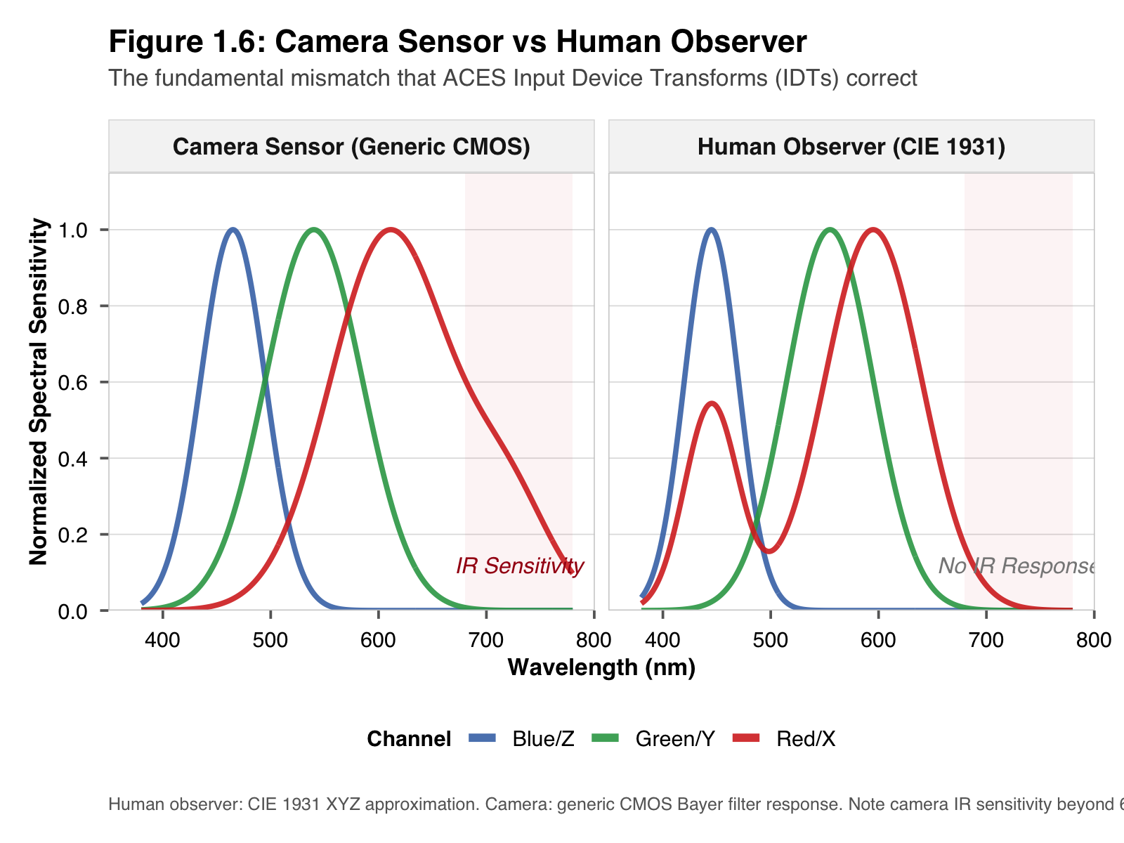
In the digital world, we replace $O(\lambda)$ (The Eye) with the Camera Sensor’s Spectral Sensitivity.
The Problem: Silicon is not Biological. A generic camera sensor does not match the LMS curves. When we build an IDT (Input Device Transform) in ACES, we are mathematically forcing the camera’s alien vision to match the human standard observer. But if the sensor captures data the eye ignores (or misses data the eye sees), the math fails.
Color, ultimately, is a simulation.
Next Module: We travel back to 1931 to see how scientists tried to turn this biological mess into a standard coordinate system.